

Moving or collecting data in Excel and worried there might be duplicates skewing your data? This guide will cover several methods, including using Conditional Formatting, Excel formulas, and the Remove Duplicates feature.
1. Using Conditional Formatting
Using conditional formatting to find duplicate cell values is one of the easiest methods and results in duplicates being highlighted in a colour that you choose.
Steps:

- Click and drag to select the cells where you want to find duplicates.
- On the Home tab, in the Styles group, click ‘Conditional Formatting’.
- Click ‘Highlight Cells Rules’, and then click ‘Duplicate Values’.
- In the dialogue box, you can choose the formatting for the duplicate values (like a particular font or cell colour). Click ‘OK’ when done.
2. Using Formulas
You can also use Excel formulas to identify duplicates. This method is useful if you want more control or need to identify duplicates based on specific conditions.
Example Formula:
=COUNTIF(range, cell)>1 – This formula counts how many times the cell’s value appears in the range. If it’s more than 1, it’s a duplicate.
Steps:
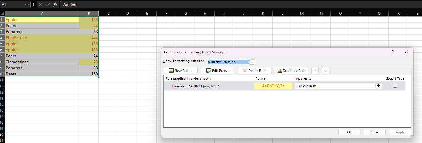
- Click on the cell adjacent to your data (to the right or below).
- Type in the COUNTIF formula.
- Drag the fill handle (small square in the cell’s bottom-right corner) to copy the formula down or across the range.
- Use Conditional Formatting (as described above) to highlight cells where the formula returns true (indicating a duplicate).
3. Using the ‘Remove Duplicates’ Feature
If you’re just looking to remove any duplicates, Excel has a built-in ‘remove duplicates’ feature to make the process really easy.
Steps:

- Click and drag to select the cells.
- On the ribbon, click on the ‘Data’ tab.
- In the ‘Data Tools’ group, click ‘Remove Duplicates’.
- In the dialogue box, specify which columns to check for duplicates. Uncheck any columns you don’t want to consider.
- Click ‘OK’. Excel will remove duplicates and show a message with the number of duplicates found and removed. If you just want to identify duplicates without removing them, you can undo this action (Ctrl + Z) after taking note of the duplicate count.Refer to the above methods to highlight duplicates instead.
Tips and Tricks
- Remember that Conditional Formatting stays with the data even when new data is added or existing data is changed.
- If checking for duplicates across multiple columns, consider concatenating the columns into one and then applying these methods.
- For large datasets, formulas can slow down Excel. Use Conditional Formatting or the Remove Duplicates feature for better performance.
- Always remember that Excel’s undo feature (Ctrl + Z) is your friend if you accidentally remove data or apply the wrong formatting.
Highlighting duplicates in Excel is straightforward once you understand these methods. Depending on your specific needs, you may choose Conditional Formatting for a quick visual reference, formulas for more complex criteria, or the Remove Duplicates feature for a fast cleanup. Remember to save your work frequently, especially when removing data.